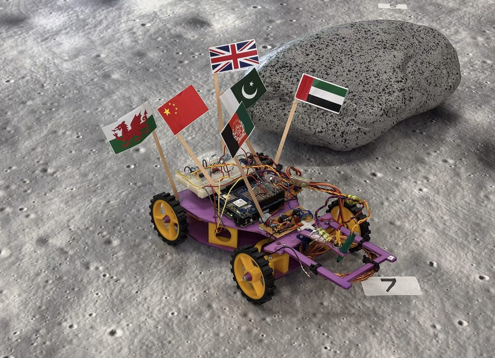
A WiFi-controlled lunar surface rover, built at Imperial College London, by six of us: Aila Danish, Hywel Evans, Beiyan Shi, Charles Wu, Saahil Zaki, and me. We designed, built, and tested it, driving across a mocked-up lunar arena, homing in on artificial “rocks,” and reading their magnetic, infrared, ultrasound, and RF signatures to classify each one.
We were awarded Best First Year Project 2026 at Imperial College London.
My part: the infrared and magnetic sensing circuits (design, testing, debugging), three of the four sensor boards soldered, and the corresponding report chapters.
System overview
The base hardware was a shared department kit: an Adafruit Metro M0 Express, a WINC1500 WiFi shield, and an H-bridge motor-driver module giving simple digital/PWM control of motor direction and speed.
A laptop-side Flask server bridges browser commands to the board over HTTP and polls it for sensor data. The finished rover is rear-wheel drive with Ackermann front-wheel steering, plus a second servo that swings a combined sensor mount (magnetic, infrared, ultrasound, and RF receivers together) to line up with a rock once the rover is in position.
Each rock embeds a magnet, an IR emitter, an ultrasound transmitter, and an RF transmitter; reading all four classifies it into one of four types:
| Rock type | IR rate | Ultrasound | Magnetic polarity |
|---|---|---|---|
| Basaltoid | High, λ=547/s | Detected | Down |
| Gravion | Low, λ=312/s | Absent | Down |
| Regolix | Low, λ=312/s | Detected | Up |
| Lunarite | High, λ=547/s | Absent | Up |
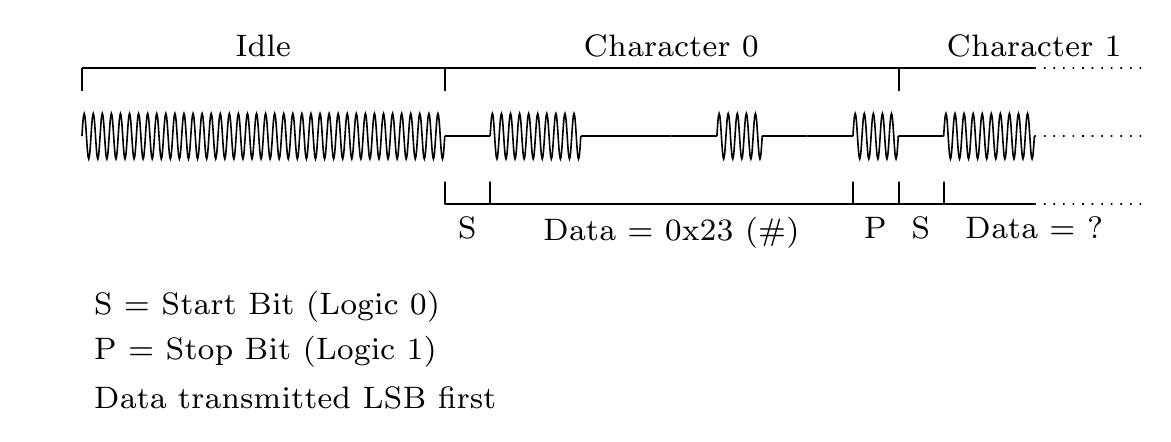
The RF signal separately carries the rock’s age, UART-encoded onto an 89 kHz carrier:
The four sensing circuits
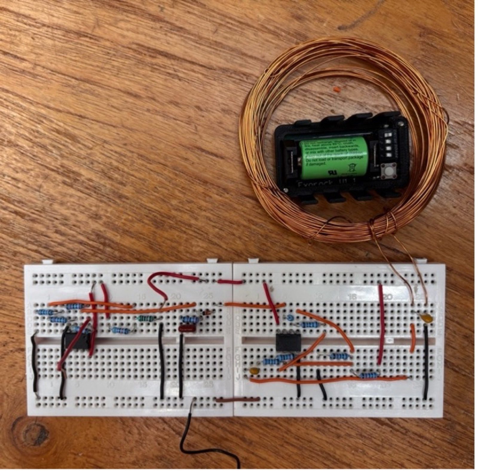
Each sensor got its own analogue front end (amplification, demodulation, and a Schmitt trigger), built mostly around the MCP6022 op-amp and proven on breadboard first.
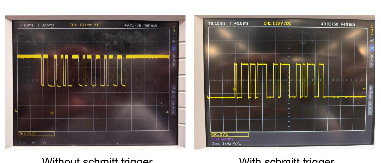
The Schmitt trigger stage earns its place at the end of every one of these chains. Straight off the demodulator, the signal is a ragged, sagging version of the original pulses, clean enough to read by eye on a scope but not something a microcontroller’s digital input can count reliably. Squaring it up with a Schmitt trigger turns that into sharp, consistent logic edges the firmware can actually pulse-count.
Infrared: the rock fires 50 µs pulses at a Poisson rate of 312/s or 547/s. Our first phototransistor (SFH300) picked up ordinary room light as strongly as the rock’s 950 nm signal and had too narrow an acceptance angle for light scattered inside the rock; the TEFT4300 fixed both. Even with the right sensor, the first working version of the amplifier chain was wrong in the other direction: it used three gain stages, presumed to be “safe” over-provisioning, and the output spent most of its time pinned against the supply rail even with no signal at all, because there was simply too much gain in the loop. Cutting it back to two non-inverting stages (~121× total) fixed that.
The other problem only showed up once the sensor was actually pointed at a lit lab bench instead of a dark box: the phototransistor didn’t just see the rock’s pulses, it also saw the room lights, and ordinary fluorescent flicker put a 50 Hz sine wave on top of everything, clearly visible on the scope after the first amplifier stage. AC-coupling the detector into that first stage (a 10 nF cap and a 10 kΩ pull-down forming a high-pass filter around 1.6 kHz) let the fast pulses through while blocking the slow, high-amplitude mains hum and the constant-light DC offset. With that fixed, firmware counts pulses over a 3-second window and classifies against a 430/s threshold, six standard deviations from both rock populations, so misclassification is essentially impossible.
Magnetic: needed field direction, not just presence, so a coil was never really an option, a coil only outputs a voltage when the flux through it is changing, and this magnet doesn’t move. We used the A1324 linear Hall sensor instead, and amplified the small deviation from a reference voltage near the 2.5 V zero-field midpoint with a 220 kΩ/4.7 kΩ differential stage, a gain of about 46.8×. In theory the sensor and reference should both sit at exactly 2.5 V with no rock nearby; in practice, measured, they came out to 2.465 V and 2.484 V. That 19 mV of real-world mismatch, multiplied by the gain, is nearly 0.9 V of offset the circuit shows even at “zero field”, which is exactly why the three output states (up ~3.1 V, down ~0 V, unknown ~2.3–3.45 V depending on how far off centre the mismatch pushes it) aren’t symmetric, and why we ended up with three classification states instead of a simple binary: a reading close to the theoretical centre is genuinely ambiguous, not a sensor fault.
Ultrasound: the Prowave 400SR100 receiver picks up a weak 40 kHz tone through the rock’s 1 mm acoustic window. The first op-amp stage works as a transimpedance front end: the inverting input’s virtual-ground behaviour converts the piezo’s tiny current output straight into a voltage across the feedback resistor, instead of trying to buffer a high-impedance source directly. A second ×30 stage brings that up further, and a slow RC rectifier (47 kΩ/1 µF, ≈47 ms) turns the 40 kHz tone into a stable presence/absence DC level instead of a waveform that needs decoding. The transducer’s narrowband response actually helped here: only a few kHz either side of 40 kHz gets through at all, so no meaningful noise showed up during testing, and the conditioned signal came out roughly 10× cleaner than the raw voltage at the transducer face. There’s a real cost to that narrowness, just not one we hit: it would make the circuit sensitive to the transmitter drifting off-frequency. Detectable up to about 10 cm from the rock.
RF: picked up purely by magnetic coupling from a coil embedded in the rock’s own PCB, no electrical connection at all. Our hand-wound coil (432 µH) forms a resonant LC tank tuned to 89 kHz (measured Q ≈ 25), which boosts the signal without smearing the UART bits riding on it. Getting Q right meant walking a line: too low and there isn’t enough gain to recover the signal; too high and the tank’s own bandwidth (roughly 2× the UART symbol rate, so a little over 1 kHz for 600 baud) gets narrower than the data needs, and bits start to blur into each other. Our first op-amp choice (LT1366) didn’t have enough gain-bandwidth or slew rate at 89 kHz to keep up; the MCP6022 did. Two ×10 stages bring the resonant tank’s output up to the amplifier’s rail limit, an envelope detector (22 kΩ/4.7 nF, chosen in LTspice before being built) recovers the UART waveform riding on the carrier, and a Schmitt trigger squares it back into clean logic. The finished chain correctly decoded a rock reporting “#933”: 9.33 billion years old.
PCB and build
All four circuits were laid out together as a two-layer board in KiCad 10, each circuit kept as its own hierarchical sub-schematic under one outer sheet, wired to a shared set of screw-terminal connectors for sensors and power. Every op-amp sits in a DIP socket instead of being soldered straight down, specifically so a faulty one could be swapped without touching solder, which mattered while we were still tuning gain values against real rocks on the bench. Laying out the actual board surfaced the usual first-PCB problems: components placed too far apart for the traces between them to look sensible, 90-degree trace bends, and power and ground routed close enough together to risk coupling noise into the analogue front ends, all fixed once the board’s ground plane (visible in blue below) went in to give return currents a short path back to source. In hindsight, a circular board would have been easier to integrate with the rest of the rover than the rectangular one we drew, mostly for its symmetry.
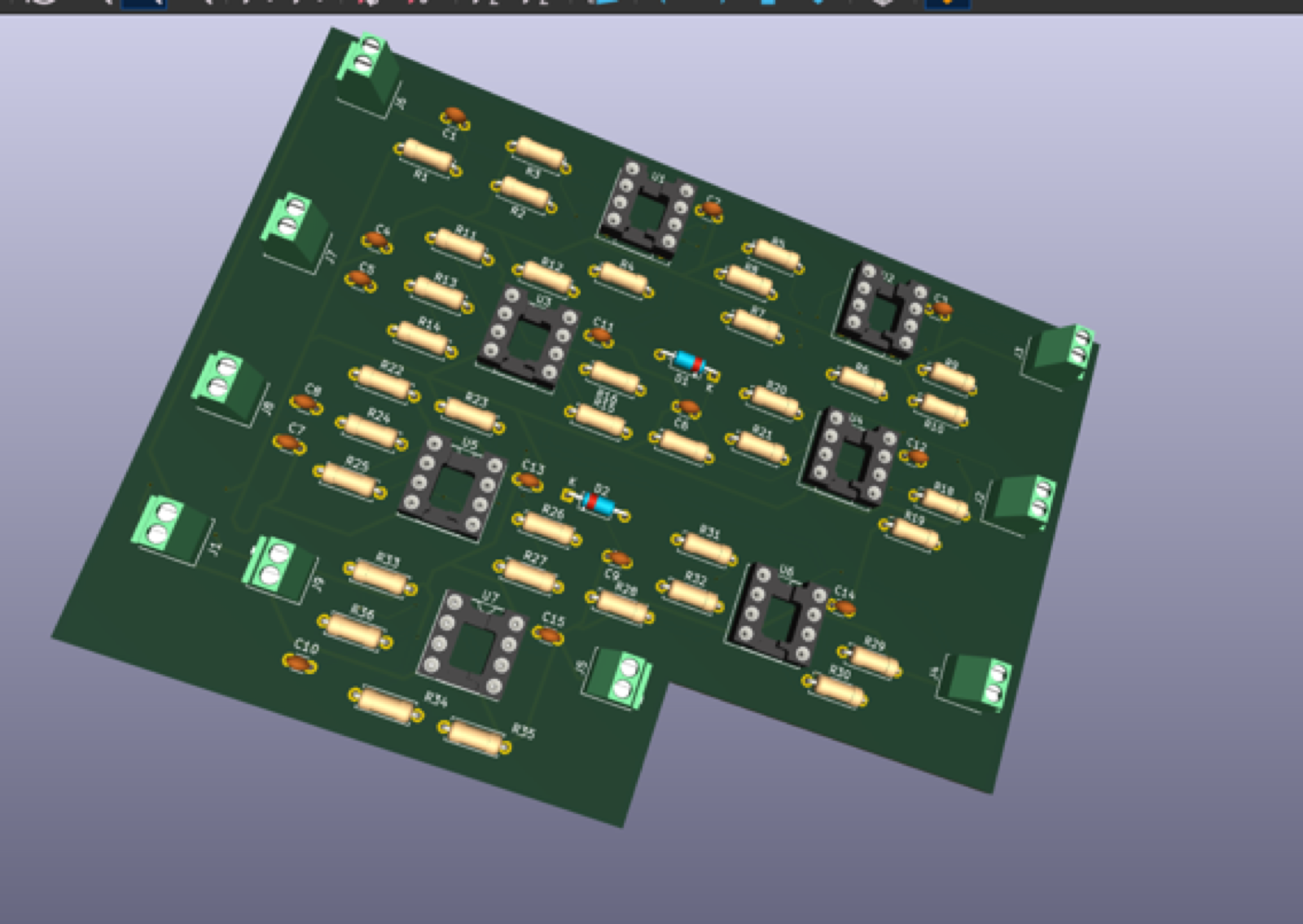
It wasn’t ordered and populated in time, though: each sensor circuit needed several more rounds of iteration than expected, especially infrared, once early testing showed how much weaker the signal was once it had to pass through the rock instead of open air, and a board on order can’t be re-valued the way a breadboard or Veroboard can. The rover that actually shipped ran each circuit soldered onto its own Veroboard module instead, a compromise between permanent breadboard and a fabricated board we couldn’t iterate on.
Chassis and drivetrain
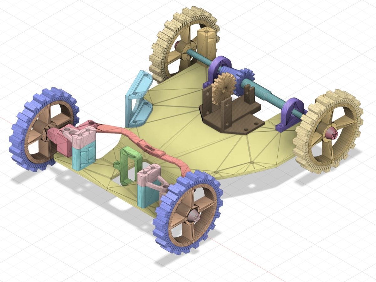
Rear-wheel drive with front-wheel Ackermann steering, chosen over the lab kit’s differential steering because differential drive couples turning to motor speed and drifts whenever the two motors aren’t perfectly matched. A single rear motor drives through a gear train; one servo steers the front wheels, a second independently swings the sensor mount to fine-align with a rock. The 3D-printed chassis (steering geometry adapted from Tim Hanewich’s open-source PYPER2) came in at 512 g, under the 750 g limit.
Software and control
Firmware on the Metro M0 runs a cooperative, poll-driven loop instead of an RTOS: each subsystem is time-sliced with millis() checks, which sidesteps re-entrancy issues since the HTTP server needs unbounded blocking time to read requests. We evaluated migrating to an ESP32 for more headroom and native WiFi, but the change came too late to fully validate, so it stayed a backup.
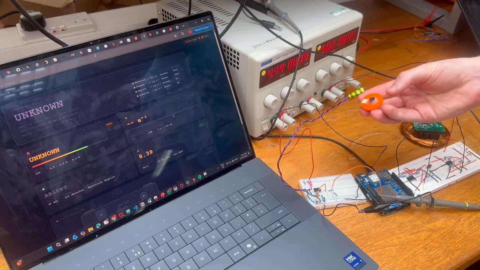
A Flask server on the laptop bridges the browser to the rover’s onboard HTTP server across three pages: a landing page, WASD manual control (Q/E for the sensor mount, R to reset it), and a live telemetry page mirroring the classification table above. We styled all three with the same dark, moon-and-earth theme instead of leaving them as bare HTML, since this was the part of the rover everyone watching would actually see on a laptop screen during testing.
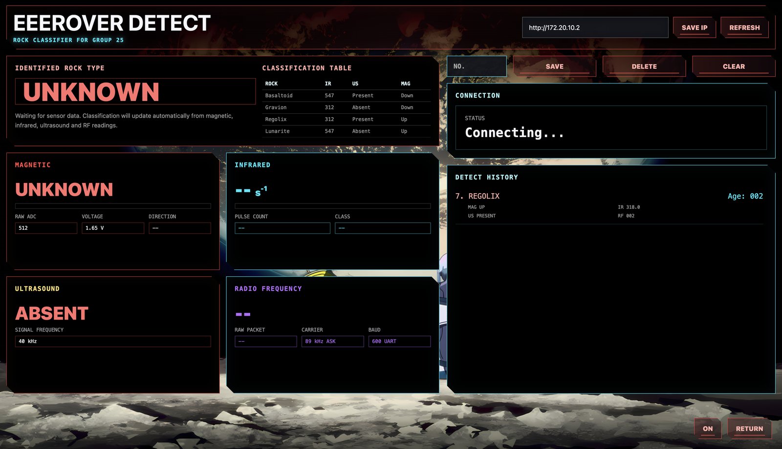
All four readings feed one truth-table lookup, where each rock type is a unique combination of IR rate, ultrasound, and magnetic polarity. It’s duplicated in the Flask bridge so the front end stays sensible even if the Arduino omits rock_type.
Testing
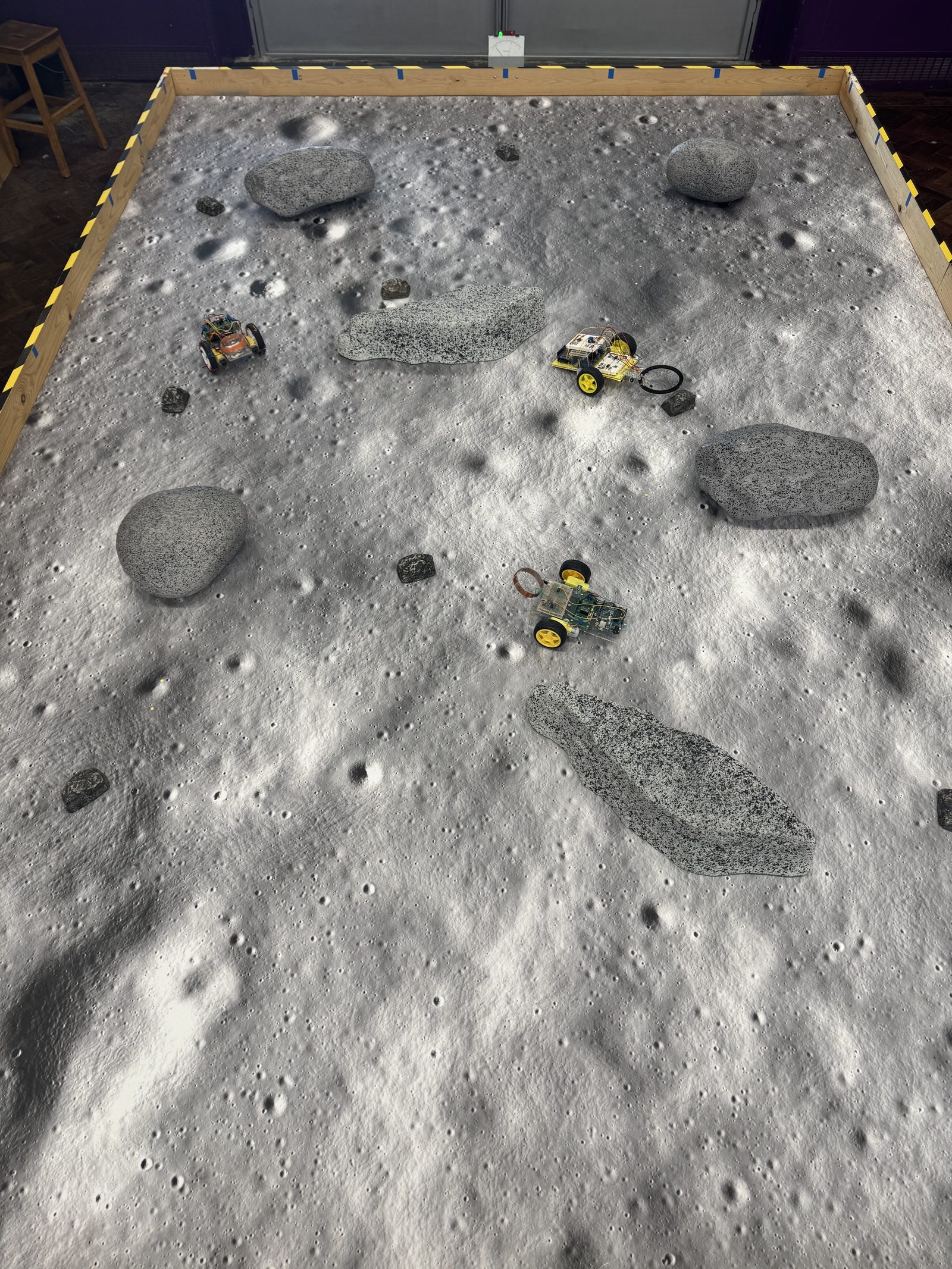
Testing happened on a purpose-built lunar-regolith-textured arena with painted foam rocks, several rovers running at once during interim sessions:
What we’d take from it
Two of us learned entire disciplines from scratch to make this work: one of the team picked up 3D printing, another PCB design, neither having done either before. Working to an actual parts budget was its own lesson, a real constraint in place of the usual unlimited university lab store. Every component swap described above (phototransistor, op-amp) came from hitting a genuine limitation on the bench, then having to justify the replacement instead of just grabbing whatever was closest to hand. Debugging faults systematically, and knowing when to stop guessing and ask a lab technician, mattered just as much as the circuit theory itself.
Team: Aila Danish, Hywel Evans, Charlie Roberts, Beiyan Shi, Charles Wu, Saahil Zaki (ELEC40006 Group 25).
Stack: Adafruit Metro M0 Express (Arduino), WINC1500 WiFi, KiCad, Python/Flask, Autodesk Fusion 360 (CAD), 3D printing.
Status: complete. Final report submitted June 2026.
Repo: private (Imperial College coursework repository).